Part 3. Need functionality in Python only available in MATLAB (e.g. Simulink)

This post is the third post on the series A trick you don’t know about Python: MATLAB.

One apparent and yet frequent reason for calling MATLAB from Python is when you need to use a specific functionality not available in Python. Such a scenario might involve using Simulink, code generation functionality, or the use of particular engineering libraries (i.e., wireless communications, controls, aerospace, biology, etc.).

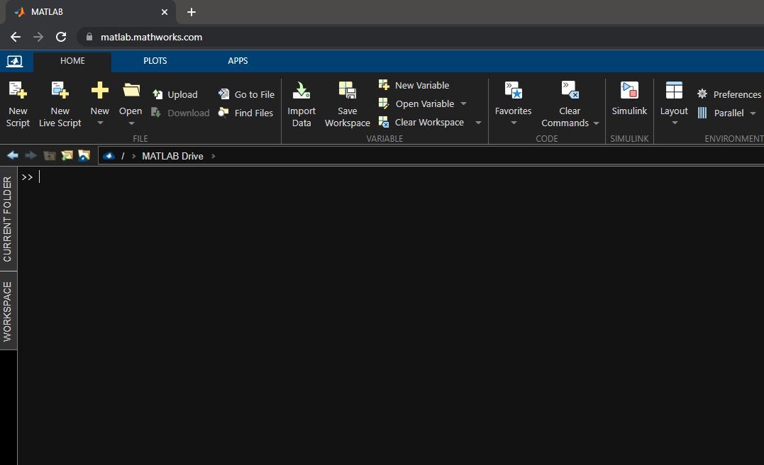
For this post, I’d like to showcase the workflow of using Python and Simulink together. As I already showed with part 1 and part 2, it all begins with starting the MATLAB Engine:

import matlab.engine
eng = matlab.engine.start_matlab('-desktop')

The MATLAB Engine API for Python provides not only access to MATLAB functions but also Simulink models:

modelName = "simulatePID"
eng.open_system(ModelName, nargout=0)

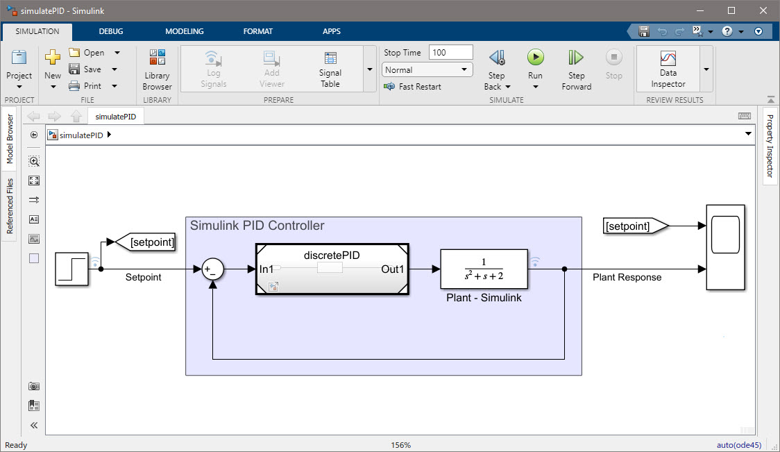
Once the model is loaded, we can send data back and forth using the eng object:

# Put variables into the workspace for the model to use
eng.workspace['Kp'] = 1.0
eng.workspace['Ki'] = 1.0
eng.workspace['Kd'] = 0.0

Running the model through the MATLAB Engine is as simple as calling the MATLAB sim function. However, I have written a function to run the model and write back the data to a Parquet file (this is another convenient way to exchange data between MATLAB and Python):

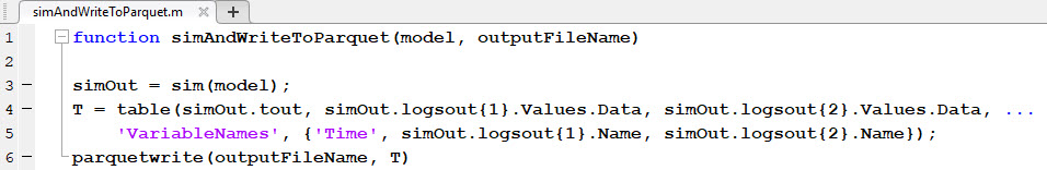
outputFileName = "controllerResponse.parquet"
eng.simAndWriteToParquet(ModelName, outputFileName)

You can then read the results from the simulation using pyarrow:

import pandas as pd
# Read as a dataframe and display
df = pd.read_parquet(outputFileName)
print(df)

     Time  Plant Response  Setpoint
0     0.0        0.000000         0
1     0.2        0.000000         0
2     0.4        0.000000         0
3     0.6        0.000000         0
4     0.8        0.000000         0
..    ...             ...       ...
248  49.2        0.999999         1
249  49.4        0.999999         1
250  49.6        0.999999         1
251  49.8        1.000000         1
252  50.0        1.000000         1

[253 rows x 3 columns]

Finally, we plot the simulation results:

pd.options.plotting.backend = "plotly"
fig = df.plot(df["Time"], [df["Plant Response"],df["Setpoint"]])
fig.show()

We can continue exploring different parameters to develop a suitable PID controller or use optimization techniques to facilitate the process and obtain an optimal set of parameters.

Once we finish, we exit the MATLAB Engine.

eng.exit()